December 6, 2020
In this blog I use my HARMONEY (“Human And Resources with MONEY”) economic growth model (also see this free early version) to demonstrate the dynamics of the Jevons Paradox: that an increase in end-use efficiency leads to an increase in total resource extraction, rate of resource depletion, and final level of depletion.
Here I summarize some important features and assumptions of the HARMONEY model to give context for why it exhibits the behavior summarized below:
- Natural resources: There is only one natural resource, and it is modeled as something akin to a forest where the resource can grow back (at some rate) after it is depleted. By this assumption, the economy can also continuously extract resources at the same rate the resources are regenerated as sort of a steady state economy.
- As resources are depleted, it takes more resources to extract the next unit of resources. This presents the ability to check the feedbacks of going after harder-to-reach resources after accessing the easiest resource first. It also allows me to calculate net energy return ratios, the so-called “energy return on energy invested” but what I will call (in later figures) the “net external power ratio”.
- Population: Population is endogenous such that population growth and decline is dependent on the level of per capita resources consumption. If there are not enough natural resources left for households to consume (per person), then population can decline and level off.
- There are 2 industrial sectors:
- The “goods” sector uses labor and capital (e.g., machines) to make new capital.
- The “extraction” sector uses labor and capital to extract resources.
- Capital requires resources consumption for
- Its operation (e.g., it needs fuel to operate)
- Its creation (e.g., capital is made out of natural resources)
- Prices: I keep the assumption from the main results in my HARMONEY paper (King (2020)) which is that prices are calculated by assuming a constant markup on the full cost of producing outputs (full cost includes wages, intermediate costs, depreciation, and interest payments).
Here I’ll focus on changing the parameter that affects how many resources are required for consumption to operate capital to produce a unit of its output. Equation (1) describes the quantity of natural resource consumption required during the operation of capital where K is the amount of physical capital, CU is the capacity utilization (a number between 0 and 1 indicating the fraction of the time the capital operates), and η is like an efficiency term, but its units are different. The symbol η represents “resources consumed per unit of capital” and its units are [resources/(time·capital)].
natural resource consumption to operate capital = η·K·CU (1)
Equation (1) holds for both goods sector operation (e.g., fuel to operate machines that make more machines) and extraction sector operation.
Demonstrating Jevons Paradox (or the backfire effect)
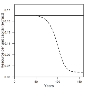
I will show a series of outputs from the HARMONEY model. There are two simulation results shown on each figure. The solid line represents the simulation where each η remains at a constant value of 0.16 throughout the simulation. The dashed line represents the simulation where each η decreases, starting at year = 50, from its maximum value of 0.16 to a minimum value of 0.0533 as a function of how fast new capital is created (e.g., rate of investment). Importantly, a decreasing η represents the SAME effect as increasing thermodynamic efficiency of an electric motor, steam turbine, combustion engine, etc. Figure 1 shows the constant η for the first simulation and the decreasing η for the second simulation.
 |
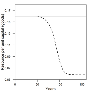 |
| Figure 1. The amount of resources consumption, or η, to operate a unit of capital in (left) the extraction sector and (right) the goods sector. Solid line = constant η (constant efficiency). Dashed line = decreasing η (increasing efficiency). | |
Figure 2 shows the amount of resources that resides in the environment, yet to be extracted. In the constant efficiency scenario, the resource can get extracted to a level of near 65 units of resources remaining (65% of its maximum possible level) at its most depleted state. In the increasing efficiency case, the resource is depleted to near half of its maximum level at about 50 units of resources remaining at its most depleted state.
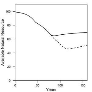 |
| Figure 2. The amount of natural resources available, or remaining, in the environment for the economy and population to consume decreases when machines become more efficient. Solid line = constant η (constant efficiency). Dashed line = decreasing η (increasing efficiency). |
Figure 3 shows the resources extraction rate that increases for the dashed line increasing efficiency scenario. (NOTE: By the definition of the resource as a forest, the maximum resource extraction rate occurs when the resource is depleted to half of its maximum level. I have chosen the parameters to not extract (much) past the 50% level for the purposes of this blog as this most accurately represents our primary use of fossil fuels.)
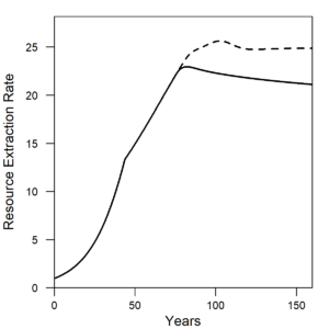 |
| Figure 3. The rate of resource extraction increases when machines become more efficient. Solid line = constant η (constant efficiency). Dashed line = decreasing η (increasing efficiency). |
Figure 4 shows a higher human population for the scenario in which there is increased machine efficiency. If a model assumes a constant or exogenous population growth, then it probably cannot exhibit the backfire effect (or Jevons Paradox). The reason that population increases with higher efficiency is that after resources are consumed to (i) operate machines and (ii) make more machines, the higher efficiency allows for more resources to be left for human consumption such that death rates remain low for a longer period of time that in turn allows population to increase for a longer period of time. Eventually, population levels off even in the increased efficiency scenario, but in a world also with more machines (more capital).
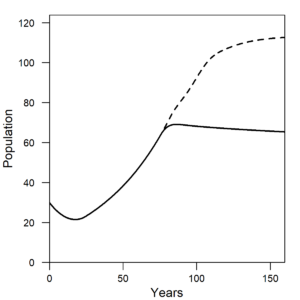 |
| Figure 4. The human population increases when machines become more efficient. Solid line = constant η (constant efficiency). Dashed line = decreasing η (increasing efficiency). |
Figure 5 shows the amount of total capital that is higher for the scenario in which there is increased machine efficiency. The reason that the capital stock increases with higher efficiency is that after resources are consumed to operate machines, the higher efficiency allows for more resources to be left for the creation of more machines.
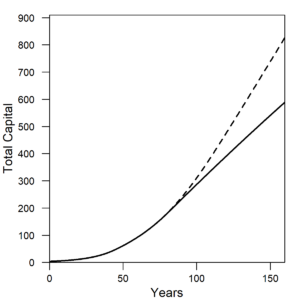 |
| Figure 5. The total capital in the economy (both for the extraction and goods sectors) increases when capital operates with higher resources efficiency. Solid line = constant η (constant efficiency). Dashed line = decreasing η (increasing efficiency). |
With increased capital, population, and resources extraction (the of the major “factor inputs” to economic production) as efficiency increases, there is also increased net output of the economy as shown in Figure 6.
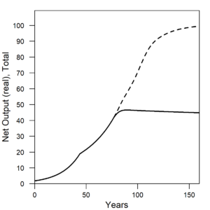 |
| Figure 6. The net output, or GDP, of the model economy is about two times larger after the increase in capital resources consumption efficiency. Solid line = constant η (constant efficiency). Dashed line = decreasing η (increasing efficiency). |
Clearly increased efficiency allows for (i) higher resource depletion, (ii) higher extraction rate of resources, (iii) an increased population, and (iv) more capital accumulation. For the latter two stocks, population and capital, higher operational resource efficiency enables more resources to be allocated to the accumulation of both more people and capital that do more work. This is consistent with the idea that more useful work, which is all energy inputs (technically exergy) times their full conversion efficiencies, goes hand in hand with more GDP. Thus, by making choices to increase efficiency in the real economy, so far (globally to date) this has translated to more useful work, resource extraction, and net output (or GDP).
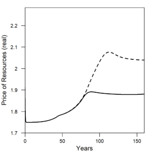
Figure 7 shows the real price of natural resources and goods (or machines). With increasing efficiency (or decreasing η in the model), the price for a unit of natural resources increases relative to a constant efficiency world, and this is precisely the trend we’ve experienced for world oil prices that increased after the 1970s, when oil efficiency efforts started. To date, oil prices have yet to return to the low prices experienced for the 90 years previous to 1974. The price of goods (or machines) decreases with the increasing efficiency in their operation.
 |
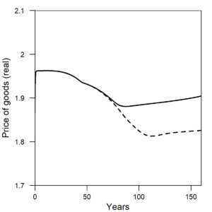 |
| Figure 7. (a) The price of natural resources increases as η, the amount of resources to operate a unit of capital, decreases. (b) The price of goods (or machines) decreases as η, the amount of resources to operate a unit of capital, decreases. Solid line = constant η (constant efficiency). Dashed line = decreasing η (increasing efficiency). | |
For the net energy geeks out there, Figure 8 shows the “net external power ratio”, or NEPR, which is the same concept that many people refer to as EROI = “energy return on (energy) invested”. (See my previous publication for reasons why I prefer to use NEPR as a more specific term.) Equation (2) expresses the idea behind the mathematics.
NEPR = (resource flows available for use outside of the extraction sector) / (resource inputs to operate extraction capital + resource inputs to create new extraction capital) (2)
When machines consume less resources for their operation, then there is period in which NEPR increases before reaching a maximum from which it again declines. This increase in tandem with increasing efficiency represents an increased net resource flow available as “net output,” which in the economic sense is that output available for consumption and investment.
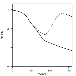 |
| Figure 8. The net external power ratio (NEPR), often referred to as EROI (= energy return on (energy) invested), increases in response to an increase in capital operating efficiency since a higher fraction of total resource flows can temporarily go to net output. Solid line = constant η (constant efficiency). Dashed line = decreasing η (increasing efficiency). |
Figure 9 shows the wage share, or percentage of GDP that is paid to wages, increases during the time that efficiency is increasing from about year = 50 to year = 110. An increasing consumption of resources and GDP can thus translate to a higher (or at least a share decreasing at a slower rate) distribution to wages.
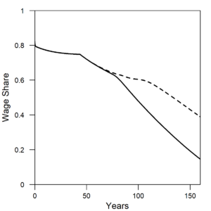 |
| Figure 9. The share of GDP that is paid to wages (or workers). Solid line = constant η (constant efficiency). Dashed line = decreasing η (increasing efficiency). |
Figure 10 shows that the debt ratio is temporarily lower while efficiency increases. Not shown (due to stopping the simulation) is that the debt ratio in the efficiency case also starts to decrease because resource constraints eventually inhibit investment below profits such that companies pay back debt. See the paper for more details. To understand the current economic situation in the U.S. and most OECD countries, it is critical to understand the context of high levels of private debt of companies and consumers (debt of consumers is not part of the HARMONEY 1.0 model). Increasing efficiency can increase output faster than debt (hence lowering debt ratio), but only for a while. Ultimately, the second law of thermodynamics limits the efficiency of energy conversations.
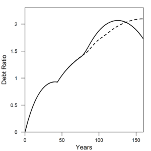 |
| Figure 10. The debt ratio (debt/GDP) of the economy increases more slowly while efficiency increases (e.g., decreasing η). Solid line = constant η (constant efficiency). Dashed line = decreasing η (increasing efficiency). |
Summary
The HARMONEY model shows many trends that are indicative of the real world economy. Thus far, globally, we keep making end-use devices more efficient, and we keep consuming energy at higher rates. When η is decreased, or efficiency is increased, in the HARMONEY model, resource extraction increases, population increases, capital increases, and net output increases. Increasing efficiency is a tactic to increase consumption and output, not a tactic to reduce overall resource consumption. The Jevons Paradox is only a paradox to those who are not thinking about the dynamics of the economy and how it responds to changes in efficiency over time.