Insights into my 2022 paper “Interdependence of Growth, Structure, Size and Resource Consumption of the Economy”
December 5, 2021
Carey W. King
This blog summarizes outcomes from my most recent publication:
King, Carey W. (2022) Interdependence of Growth, Structure, Size and Resource Consumption During an Economic Growth Cycle, Biophysical Economics and Sustainability, volume 7, Article number: 1. Free online access: website link and pdf.
Background
The purpose of this paper is to discuss the dynamic interdependencies among growth, size, and structure of an economy using outputs from an updated version of the Human and Resources with MONEY (HARMONEY) model that was published in 2020. This new version is HARMONEY v1.1.
Because of its structure, the HARMONEY model helps “narrow the differences” between economic and ecological viewpoints, which as the late Martin Weitzmann suggested, provides value by creating enhanced understanding of economic dynamics. That is to say, because the model simultaneously tracks physical and monetary stocks and flows, by including physical resources and constraints along with macroeconomic accounting and debt, HARMONEY speaks the language of both economists and physical and natural scientists.
I summarize the following insights from the paper:
- Insight #1: Efficiency begets more consumption and accumulation, not less (Jevons Paradox)
- Insight #2: Economy Shows Same Energy-Size Scaling as Biological Growth
- Insight #3: Enhanced Interpretation of Decoupling Resource Consumption from GDP
- Insight #4: Labor (wage share) vs. Capital (capital share) vs. Resource Consumption Tradeoff
- Insight #5: Evolution of Economic Structure and Complexity
See below for “How the Model Works” and of course you can read the full paper for free.
Insight #1: Efficiency begets more consumption and accumulation, not less (Jevons Paradox)
One of the frustrating aspects of reading most journal papers and discussions of economic modeling is the treatment of the concept of energy efficiency. Given the HARMONEY v1.1 assumption that higher profits translate to increased investment, increasing energy efficiency clearly enables increased natural resource depletion (Fig. 1a), while enabling the economy to achieve higher resource extraction rates (Fig. 1b), population (Fig. 1c), capital accumulation (Fig. 1d), and net output (or GDP, not shown). In other words, the HARMONEY model supports the Jevons Paradox, or backfire effect, in that higher fuel efficiency in operating capital increases overall economic size and consumption. This theoretical finding is consistent with studies supporting the evidence for a strong rebound effect, as well as the general observation that over the course of industrialization to date, the human economy has indeed invented and employed more efficient processes while at the same time consumed more energy decade to decade.
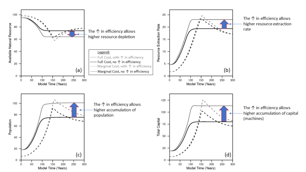
Figure 1. HARMONEY shows how increased resource efficiency of capital (e.g., as fuel) enables more growth and resource depletion.
Insight #2: Economy Shows Same Energy-Size Scaling as Biological Growth
Figure 2 (Figure 4 in the paper) demonstrates an additional explanation of the relationship between natural resources consumption and growth by making an explicit comparison to biological growth. Figure 2a compares a typical metabolism versus mass trend (for a cow starting from birth per West et al. 2001) to corresponding results from the HARMONEY model. Here I’m explicitly comparing two things.
First, an animal’s metabolism compares to the natural resources consumption in HARMONEY, and to total primary energy consumption in the real world data: animal metabolism compares to economy energy consumption.
Second, animal mass compares to physical capital (like cars and buildings) in the economy: animal mass compares to economic (physical) capital. In the real economy there is a problem with adding up all the capital, but that is a much-discussed longer story, so I won’t go into that here. Thus, most existing studies that make the economic-biological growth comparison plot primary energy versus gross domestic product (GDP), which is not as consistent of a comparison. However, in HARMONEY, capital is a well-defined concept that can be summed consistently so I plot resource consumption versus both capital and GDP.
Figure 2a displays curves for an animal (e.g., a cow) total metabolic power and basal metabolic power, scaling with mass to the 0.5 and 0.75 power, respectively. The difference between “total” and “basal” is the metabolic power allocated to growth of new mass (shown at the bottom of the chart). One important point is that most organisms grow only to a certain size, with the trajectory of Fig. 2a moving up and to the right, eventually stopping at some point (indicated by the big red dot). The HARMONEY scenarios (assuming full cost pricing) show the same type of trajectory.
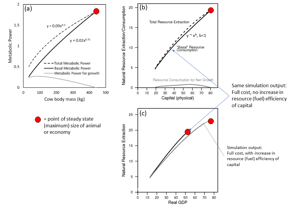
Figure 2. A comparison of patterns between (a) biological growth (metabolism and mass) and (b and c) economic growth (natural resources consumption and (b) capital and (c) GDP.
Figures 2b and 2c show the full cost pricing simulation for HARMONEY to compare to biological growth. Just like in growth of an animal, the economy grows until a point at which it stops and remains at a steady state value of resource extraction, GDP, and capital. Also, total and “basal” metabolism (for animals) and resource consumption (for the economy) come together at the end of growth (which is pretty much the definition of the end of growth).
Figure 2c shows the gray line from a simulation which assumes increases in resource efficiency of capital (like fuel efficiency, same as results in Figure 1). Again, you can see that the final values of GDP and resource consumption rates are higher if the economy can operate capital at higher efficiency. We can also see that the resource extraction scales pretty similarly to both capital and GDP. It is an open question as to how insightful it is to relate economic metabolism to GDP instead of capital; perhaps both are useful.
Insight #3: Enhanced Interpretation of Decoupling Resource Consumption from GDP
This paper has much to say on the issue of relative decoupling defined as increasing GDP faster than increasing resources consumption. Decoupling can be envisioned by plotting data as in Figure 3 which shows the growth rate (e.g., the rate of increase) of energy and resources consumption versus the growth rate of GDP. Global data use real gross world product (GWP) and global primary energy consumption.
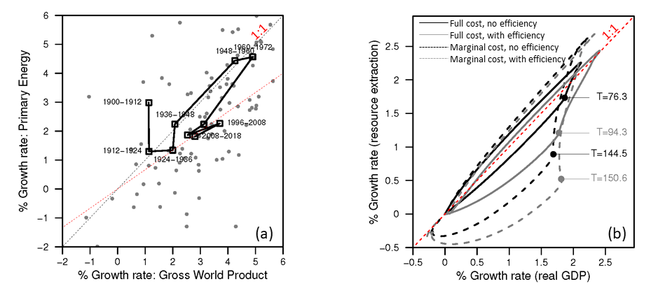
Figure 3. (a) Global data showing the growth rate of primary energy consumption versus growth rate of real gross world product. (b) Comparable data from the HARMONEY model for growth rate of resources consumption versus growth rate of GDP.
Relative decoupling occurs when the growth rate data are below the 1:1 sloped line, in the shaded area (Figure 4).
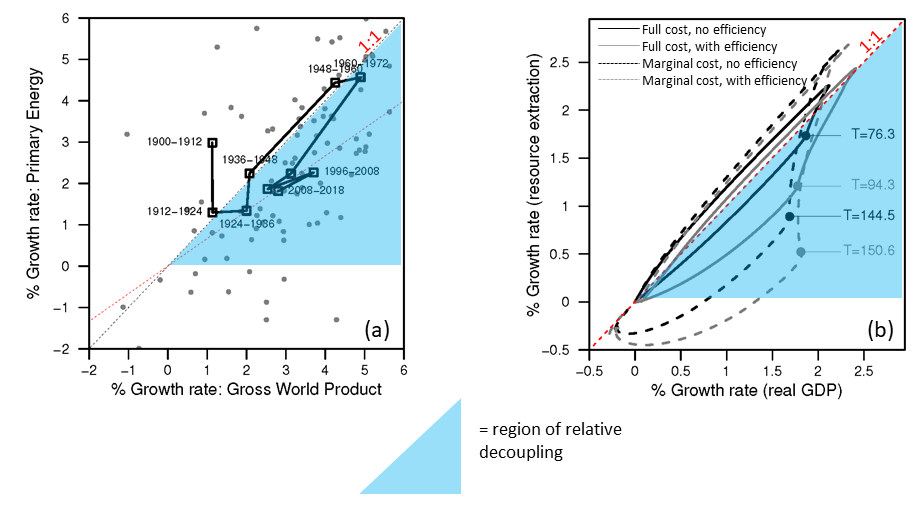
Figure 4. Relative decoupling occurs when the growth rate data are below the 1:1 sloped line, in the shaded area.
Figure 5 shows that both the global data and the HARMONEY simulations show the same temporal trend which is to move in a clockwise direction in the figure. First the both energy and resources consumption increases at nearly the same rate as GDP, and they both increase growth rates (which is to say grow faster over time). This is to say the growth rates move up and to the right along the 1:1 line. Second, once growth rates no longer increase, they move down and to the left into the relative decoupling zone. For the global data since the mid-1970s, GWP has grown at about 3%/year and primary energy consumption at about 2%/year.
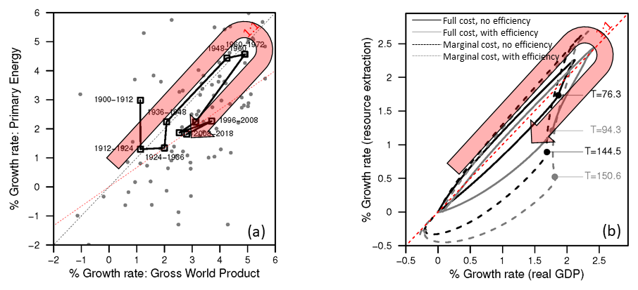
Figure 5. Both the (a) global data and (b) HARMONEY simulations show the same clockwise trend over time.
One important interpretation of this trend in growth rates goes against how most people think of the role of energy efficiency in relative decoupling. A common interpretation of relative decoupling is that it occurs because the economy becomes more efficient in its consumption of energy in producing the goods and services of which GDP is composed. However, when the HARMONEY model results reside in the decoupling zone, there is no change in any parameters of the model that can be associated with resource efficiency! In fact, the opposite is the case: due to resource depletion, in the relative decoupling phase the dominant feedback is one of decreasing efficiency in that more resource consumption is required to extract a higher rate of resources.
The HARMONEY model moves from the 1:1 “full coupling” line to the relative decoupling zone because the GDP and resources consumption can no longer increase at increasingly high rates. That is to say, not only does a stage of relative decoupling occur during periods with no perceivable increase in device energy efficiency, the shift to this stage of growth is evidence for limits to growth, not evidence against limits to growth. In HARMONEY v1.1, resource limits eventually constrain growth to go slower, and eventually go to zero, due to the definition of the forest-like natural resource in the model.
However, this is not to say that increasing resource efficiency is completely unassociated with higher levels of relative decoupling. Figure 6 shows that increasing the resource consumption efficiency of machines, the economy can move more deeply into a state of relative decoupling.
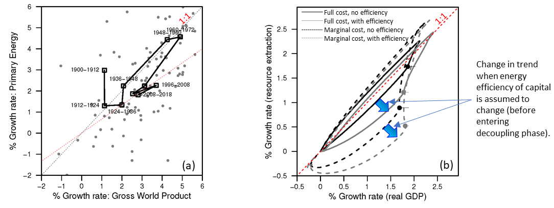
Figure 6. HARMONEY results highlighting that while relative decoupling is not definitively associated with increasing resource efficiency, an increase in resource operating efficiency of capital does move the results more deeply into relative decoupling.
Insight #4: Labor (wage share) vs. Capital (capital share) vs. Resource Consumption Tradeoff
Income inequality has been foremost in the minds of many people for the last 10-15 years. The contemporary explanation is that there is a battle between “labor” (wages) and “capital’ (profits). One way to measure this “battle” is to compare the share of GDP gong to wages (wage share) versus profits (capital or profit share).
The claim is that since the 1970s workers have lost “bargaining power”, or the legitimacy and support to ask for higher wages, largely because of the decline in support (including from elected officials) for union membership. I tested this idea in this paper, and the HARMONEY supports this general premise, but suggests there is more to the story: resource consumption rates.
I model workers having full bargaining power when their wages can increase with inflation. Figure 7 shows that wage share declines during the growth phase as companies acquire some profit share. However, once resource extraction rates level off (refer back to Figure 1), wage share rebounds back to its initial higher level and profit share declines to zero.
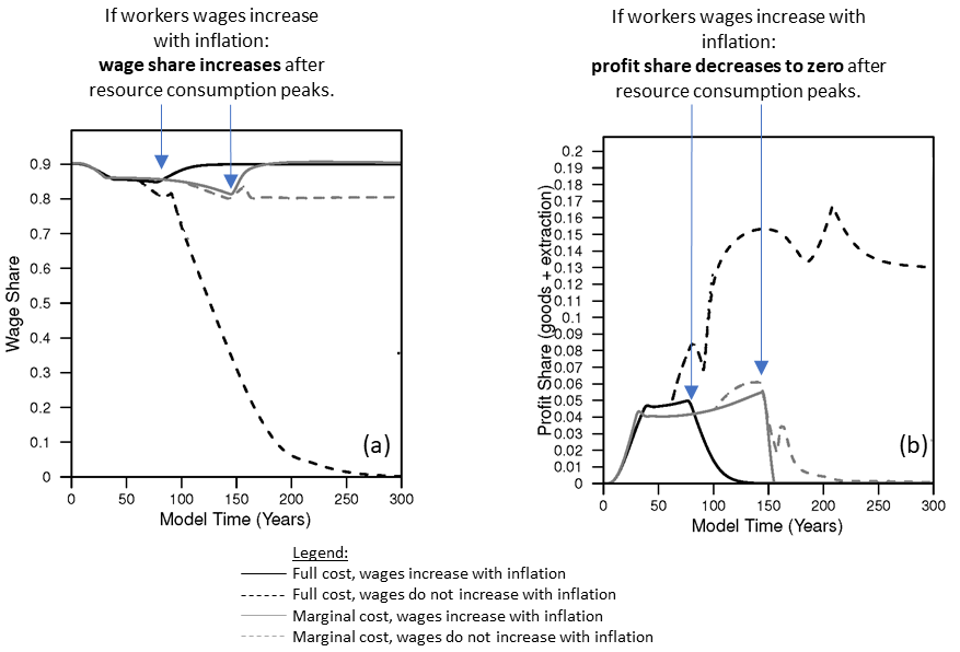
Figure 7. When resource consumption rates peak (and no longer increase), and when workers can bargain for wages, (a) wage share (the fraction of GDP going to wages) can stay high and rebound while (b) profit share of companies declines to zero.
Figure 8 shows that if we slowly remove bargaining power (by no longer allowing wages to increase with inflation) when resource extraction per person peaks (just as the trend begins in the U.S. economy), then wage share either declines (for the “full cost” scenario) as companies continue to invest in capital or wage share remains low (for the “marginal cost scenario). See the full paper for descriptions of two different assumptions for production costs.
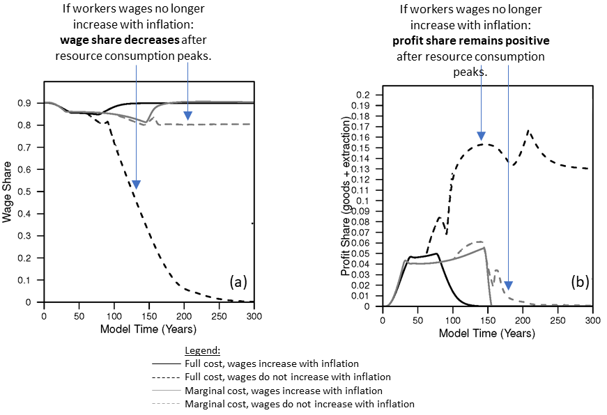
Figure 8. When resource consumption rates peak (and no longer increase), and when workers can bargain for wages, (a) wage share (the fraction of GDP going to wages) can stay high and rebound while (b) profit share of companies declines to zero.
These results show that nature of the distribution of economic proceeds changes once the economy stops growing. As one might guess, it is harder to make profits in a time a stagnant energy and resource consumption rates, and in the face of that slowdown or stagnation, profits can be maintained with the sacrifice of wages. The HARMONEY model suggests this might be what happened to U.S. labor starting in the late 1970s and early 1980s. Yes Ronald Reagan was elected President and he was a “union buster”, but we might also ask about the forces that propelled Reagan (and other business friendly legislators) to office and supported a reduction in labor-friendly policies.
Insight #5: Evolution of Economic Structure and Complexity
In a 2016 paper (pre-print and blog) I tracked the changing dynamic structure of the U.S. economy since 1947 using (information theoretic) metrics that quantify the distribution of the flow of money within the economy (specifically the input-output “Use” tables). In Figure 9 I show two images that summarize some of the simulated HARMONEY scenarios as compared to the calculations from the U.S. data.
Figure 9a provides two metrics (mutual constraint & conditional entropy) that when added together form a third metric (information entropy) that is plotted in Figure 9b.
Why should we care about these metrics? Many people view information entropy as a metric of complexity. Higher information entropy means higher complexity, where complexity in the economic context means the economy is performing a more diverse set of activities with each activity associated with more equal contributions.
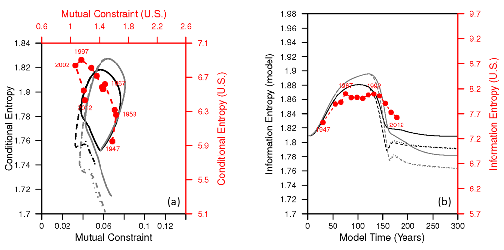
Figure 9. Information theoretic metrics that quantify the internal structure of the economy over time. The data with large red circles and dashed lines show calculations from my previous 2016 paper. The lines without circles are simulated trajectories using HARMONEY v1.1. NOTE: mutual constraint + conditional entropy = information entropy.
Figure 10(a-left) shows that both the U.S. data and the HARMONEY simulations show a counter-clockwise pattern during an expansion (fast-growth phase) that eventually leads to a slower-growth phase (after 1997 in U.S. data).
Figure 10(b-right) shows information entropy over time, and both the U.S. data and the HARMONEY model show three successive trends from increasing to constant to then decreasing information entropy. Importantly (the paper describes more fully) the change in trends in Figures 9 and 10 relate to changes in both (i) the rate of resources (or energy) consumption and (ii) the cost of energy. That is to say there are similar reasons why there are changes in trends in Figures 9 and 10 for both the U.S. economy and the HARMONEY model.
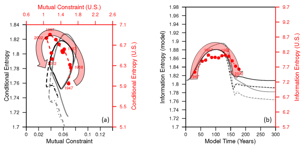
Figure 10. Same as Figure 9 but with added red shaded arrow to emphasize the broad trend.
The comparison on Figures 9 and 10 provides evidence that HARMONEY accurately represents internal changes in structure and complexity of a real-world economy during a growth cycle.
Conclusion & Takeaways
The key takeaways are that both animals and the economy require energy consumption and resource to (1) operate their existing mass and capital, (2) make new mass and capital, and (3) distribute and acquire energy. If you put these concepts into an economic model, as done in HARMONEY, you are a big step towards enabling your model to realistically describe energy-economic interactions. This type of consistent modeling is important, for example, for the modeling of a low-carbon energy transition. A low-carbon transition will very likely require major shifts in economic structure due to shifts (downward) in energy efficiency (think CO2 capture plants) and increase allocation of resources to make new capital (such several terawatts of wind, solar, and battery capacity across the globe). I continue to work on HARMONEY to inform the structural dynamics of economic growth in ways that are not possible using the usual (e.g., neoclassical growth) methods.
How the Model Works
HARMONEY v1.1 is a system dynamics model centered on simulating a set of ordinary differential equations using stock-flow consistent tracking of monetary flows. HARMONEY v1.1 is still a toy model, which is to say it is not yet calibrated (we’re working on it!) to a real economy, such as the United States. Nonetheless, it has critical features and structural assumptions that make it applicable and valuable for comparing its trends to long-term trends in real-world data.
This is to say, an important part of HARMONEY is that it has a conservation of flow principle for both mass (as physical resources, energy or minerals, extracted from the environment) and money (at any given instant flows of money are tracked between firms, households, and private banks). While this idea has been around for many decades, this is still relatively unique for macroeconomic models.
Here are several assumptions in the design of the model that help explain why it can mimic long-term real-world trends relating energy consumption and economic variables
- The resource that supports the economy is a regenerative renewable resource stock, such as a forest.
- Resource (mass, energy) consumption is required for three purposes in the model, just like the real world:
- To operate machines (as fuel)
- To become new machines when they are manufactured (embodied in new capital)
- To “operate” or feed people to keep them alive (as food)
- Money is effectively defined as all of the following
- the compensation labor (workers) receive,
- the profits received by companies,
- money (as credit) is created when banks give loans to companies to invest in capital at levels beyond their profits, and the money is destroyed when companies pay back debt, and
- the interest payments on the debt, or loans given to companies.
- There is no government in the model.
- Population declines when there is not enough resource consumption for households.