In my last macroeconomic modeling paper I compared my model outputs to the long-term pattern in global energy and GDP data (see my blog discussing the main takeaways).
The energy data were arranged by colleague Andrew Jarvis as we discussed in this pre-print paper (a revised version again in peer review). The data we discussed were those relating global primary energy consumption to real gross domestic product (GDP) of all countries (see Figure 1, left).
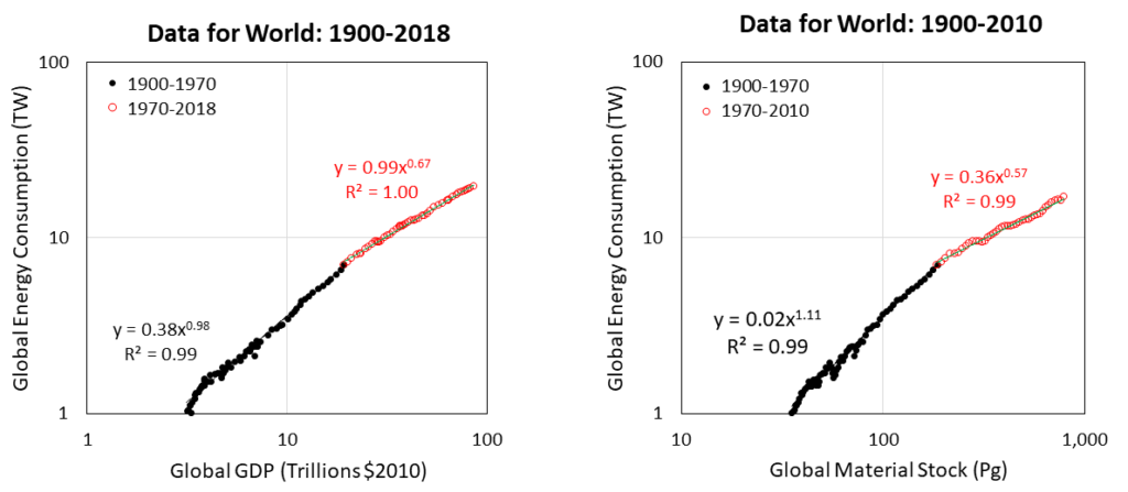
Figure 1. (Left) Global primary energy consumption vs. global gross domestic product (log-log axes). (Right) Global primary energy consumption vs. global material stock (log-log axes).
One very interesting feature of these data is that from 1900 to about 1970, there is one pattern in Figure 1, but after 1970s there is a different pattern. That is to say, as indicated by the change in slope of the time series of data, the global economy seems to have operated in one manner leading to the 1970s, and in a different manner ever since.
There are two interesting questions relating to this feature, or change in trend in the 1970s. First, what was fundamentally different about the years before the 1970s versus after the 1970s? Second, are there existing ideas that can help us explain this change in pattern?
I discuss the second question first.
Many scientists have discussed a similar relationship in biology as we see in Figure 1. Single-celled organisms (eukaryotic cells, like amoebas) grow in a near linear manner relating energy consumption and their mass (or size). If you have a 2 times bigger cell, that cell needs 2 times more energy consumption. In a similar way, before 1970, when the global economy got 2 times bigger, it consumed 2 times more energy. We call this “linear scaling”.
However, when scientists analyze multicellular organisms, including mammals, they tend to find “sublinear scaling.” Thus, a rabbit that is about 10 times more massive than a rat does not consume 10 times more energy, it consumes about 5-6 times more energy since mammal basal metabolism scales with mass to the 3/4 power — (10 times more mass)3/4 = (5.6 times more metabolism). This trend for mammals is named Kleiber’s Law, and metabolism scales “sublinearly” with mass because the exponent 3/4 has a value less than 1. The same type of sublinear scaling also occurs for “superorganisms” composed of many individuals, such as with ultrasocial insects like ants and termites.
Thus, in a similar was as seen in biology, the global economy transitioned from linear scaling to “sublinear” scaling in relating energy consumption and size. Before 1970 global energy scales approximately linearly with GDP, or E ~ GDP1, when 2 times more GDP required 2 times more energy consumption. But after 1970, energy consumption scales sublinearly with GDP, at approximately E ~ GDP2/3 such that when GDP increased 3-fold, energy consumption increased by only about 2 times.
So there seems to be a very nice parallel in growth patterns between biological organisms and the global economy. In smaller organisms and a smaller global economy, energy consumption increased linearly with size, but in larger multi-celled organisms and a larger global economy energy consumption increased more slowly than size.
However, note one problem with the comparison so far. The left image of Figure 1 uses GDP as the metric for size, but in reality it is not the best analog metric for animal mass because it has units of money per time. GDP is a metric for a flow of output (this output measured as money per year). It is not a stock of accumulated mass representing the physical size of the economy in an exact parallel to biological organisms.
However, we do have estimates for the mass of the economy. Fridolin Krausmann and co-authors produced an estimate of the mass of accumulated materials in the global economy from 1900-2010. These materials include such categories as wood, metals, plastics, concrete, bricks, sand, and gravel. The right side of Figure 1 shows the pattern when we plot the same global energy consumption data versus the accumulated mass of the economy (in petagrams, or Pg, where 1 petagram = 1015 grams = 1 billion metric tonnes).
The right image of Figure 1 indicates the same basic pattern as the left image of Figure 1, but here the x-axis is MUCH MORE analogous to mass of biological organisms. Here the scaling of energy to mass before 1970 is about 1.1, meaning that when accumulated economic mass increased 2 times, the energy consumption increased more than 2 times as much (say 21.1 = 2.1 times more).
After 1970, the scaling of energy consumption to mass is 0.57 (as opposed to about 0.67 when scaling energy consumption to GDP). Thus, when the accumulated mass increased 2 times after 1970, energy consumption increased by only about 1.5 times.
You might ask about the mass of humans and livestock that are also part of “the economy”, but the total dry mass of ourselves and domestic animals is less than 1 Pg today, so our biological mass doesn’t change the data in Figure 1 in any significant way.
Now back to the first of our main questions about the change in trend in the data in 1970. What was fundamentally different in the economy in the years before the 1970s versus after the 1970s? Also, is there parallel explanation in biology?
My hypothesis, informed by biological literature, my macroeconomic modeling, and economic data suggest to me that both of the following effects started to dominate in the 1970s: (1) energy extraction became more expensive (in money and in terms of energy inputs), and (2) the world increased the distribution of materials among countries.
First, peak oil production in the U.S. in 1970 (yes, U.S. oil production in the last decade has since surpassed the peak in 1970), and the rest of the developed countries (e.g., Europe, Japan, Australia, New Zealand) forced a slowing of growth rates due to energy input constraints. Oil has been more expensive since 1973, averaging about 63 $/BBL since that year, as compared to about 21 $/BBL for the previous 90 years.
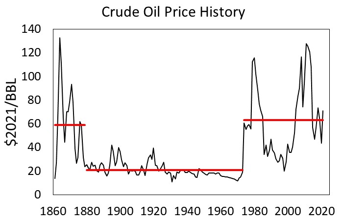
Figure 2. Global oil price history in real dollars per barrel ($2021/BBL). [BP Statistical Review of World Energy]
My “HARMOMEY” macroeconomic model shows that an economy relatively unconstrained by natural resource (e.g., energy), such that it can growth increasingly fast, has near linear or superlinear scaling of resource consumption to size. However, once an economy becomes constrained in its ability to consume energy at higher rates, it has the tendency to move from a phase of linear (or superlinear) scaling of energy consumption to GDP to a new phase of sublinear scaling (see Insights 2 and 3 in my previous blog). The earlier linear phase of growth occurs when the system (biological organism or economy) is not constrained by energy access, and it cannot perceive a boundary to its growth (the exponential growth phase). It is instead constrained by the number of structures that are able to consume the energy. Eventually, the system grows to sufficient size that it notices a limit to its resource access, the rate of energy extraction slows, and it begins to create new subsystems or levels of cooperation to access more costly (in time, space, and energy input requirements) resources.
This leads to the second possible reason for sublinear scaling after the 1970s: globalized trade. Once the major world economies could no longer easily increase oil production at a whim within their own borders, there was an increased need to acquire and distribute resources (e.g., oil) and manufactured goods across the planet. World Bank data show that in 1970, the value (in money) of international trade was 25% of global GDP, but in 2008 it was 61%, and it has resided between 50% and 60% since.
This increase in costs and structures for both acquiring energy and distributing materials occurs when organisms become multicellular, and different sets of cells begin to take on specialized functions, or tasks (e.g., heart muscle cell versus a liver cell). Larger biological organisms require more movement, or locomotion, to acquire food, and they develop networks to internally distribute nutrients within their bodies (i.e., blood circulatory system) just like the global economy had to develop new networks to internally distribute resources among countries.
As stated by DeLong et al (2010): “Metabolic rates of metazoans [small multicellular aquatic animals] initially tend to increase linearly with number of cells and body mass, but as vascular systems evolved to distribute resources to increasingly large bodies, geometric constraints required sublinear scaling, converging to the 3/4 power scaling of Kleiber’s law …”. We can viably argue that there were similar “geometric” constraints that became more prevalent upon the global economy starting in the 1970s. While the Western industrialized countries still dominated global GDP in the 1970s and 1980s, in order for the global economy to grow there was a greater imperative for more interconnection via an economic “vascular” system. We call this globalization.
In summary, the global economy and biology have very parallel growth patterns relating energy consumption to size. It is critical more leaders and citizens understand the patterns described in this blog because most economic models are incapable of explaining these growth patterns. This means both that most economists do not know why these most fundamental patterns exist and therefore their advice, derived from models and economic frameworks, cannot accurately inform public policy or corporate strategy.
This type of research and understanding also informs important questions related to the feedbacks, costs, and benefits from reducing greenhouse gas emissions at a given rate (the rate matters!) as well as whether we can decouple economic growth from material and energy consumption (it is unlikely). I and others within the communities of biophysical economics (BPE Institute, ISEOF, Exergy Economics) and ecological economics (ISEE, USSEE, ESEE, etc.) are working on more accurate economic models that can inform this and other pressing questions (equity, debt, etc.). Watch my latest talk (September 2022) at the Fields Institute in Toronto.